Timing accuracy is of paramount importance for occultations observers, but also astrometrists should worry about it when measuring positions of objects like fast NEOs (Near Earth Objects). It is not unusual, indeed, that on MPC’s NEO Confirmation Panel (NEOCP) appear very quick objects, moving at a rate exceeding 100″/minute (1,7″/sec). These asteroids are tentalizing for the observer because often are very bright (mv around 17 or less) but, on the other side, they pose a serious problem in positional measurements because timing errors can be not negligible here. Consider an asteroid moving at 120″/min (2″/sec), this implies that an error of only 0.1 sec in timing translates into a positional error of 0.2″, about two times the accuracy you strive to reach when measuring slower asteroids. Note that timing inaccuracies are only a part of the story, and adding to all other sources of error affecting astrometric measures (bad guiding, high residuals of reference catalogue stars, unfair seeing etc) it is not unusal your residuals raise to more than 1″, being then rejected by Minor Planet Center, which of course you do not want to.
Step 1: synchronize your PC
In order to solve the problem, first of all you need to set up a good synchronitazion between your PC and a reliable source of timing. This can be done in various ways:
- using a NTP server (SNTP is a simpler and less accurate protocol) which sends the correct time to your PC clock;
- using a GPS camera;
- using a GPS device which can interface with your computer directly.
The first method is in general cheap (or free), and can be a good choice if you use a reputable software. I personally used Meinberg (after some year with Dimension-4 which still relies on SNTP protocol), that you can download from here; in addition, you want to check the status of the server via the Meinberg monitor. The use is very simple, just disable/uninstall any similar software (check expecially your Windows synchronization settings in order to avoid conflicts), then Meinberg takes care to connect to the best time server, synchronizing your PC’s clock with a frequency set by the user. In practice, you don’t need to do anything except periodically check the NTP Status, which displays the delay, jitter, and error in milliseconds (offset). See screenshot below.
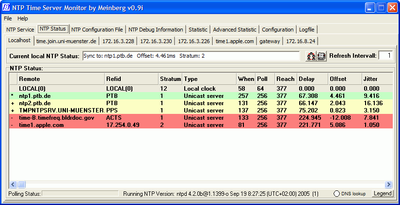
Screenshot from Meinberg NTP Status Monitor
These two tools can give you a synchronization probably around 0.1 seconds, which is just very good, but basically you need an internet connection (not a problem in many Observatories though). More important, the mandatory internet connection itself is not always stable, and this means your accuracy varies over time. You can check your timing errors with several internet websites (I use https://time.is/), but do not blindly trust them!
The GPS cameras are probably the best solution overall, but I am not going to discuss them here as they are very expensive and generally reserved to occultations enthusiasts.
The last method we discuss here consists in a GPS antenna, which can receive absolute time from GNSS satellites (equipped with atomic clocks) and send it straight to your PC clock. There are various devices on the market, in my Observatory (MPC code D43) I personally use the TimeBoxII by Shelyak Instruments. It is not exactly cheap, say like a good eyepiece, but it costs much less than a GPS camera and can be also used for occultation work. The use is very intuitive; just plug in the box, bringing the supplied antenna outside so it can reach the satellites. When they are enough, the control panel indicator becomes green and the box starts synchronizing your clock with an accuracy of the order of milliseconds. The number of satellites in sight, together with the difference between absolute time and PC time is always displayed (see capture below).
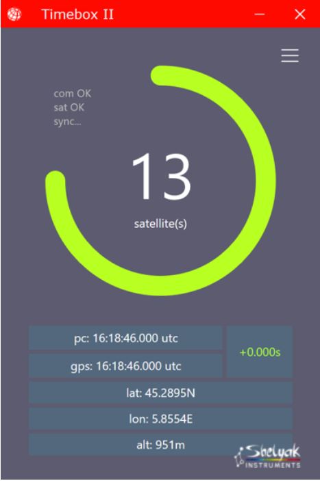
The TimeBoxII control panel
Step 2: calculate your timing delay
Having a good PC time it’s very important, but one should not forget that what matters (and what you send to Minor Planet Center) is the observing time, written in the DATE-OBS field of the FITS files of your astrometric session. To keep it simple, when an exposure is over, the software controlling your camera (e.g., SharpCapture) receives the data from it and calculates the relevant DATE-OBS, which in general is the start of the exposure. But unfortunately the software has no idea of when the data are leaving the camera itself and can only record when they arrive, hence it is important to calculate this delay in order to properly compensate for it.
You can use the PPS (pulse per second) provided by the TimeBox led together with timestamps, or, more easily, rely on the GNSS satellites (see Bill Gray website for insights on the method). In short terms, you need to measure the positions of such a satellite, just as you were measuring a fast NEO. It’s not a problem to find one, as in general you always have a dozen upon your horizon and the Bill Gray’s website provides accurate ephemerides for them. They are in general very bright (around magnitude 1o-11) and very fast, so you need a very short exposure time if you do not want to deal with long streaks. In general I use not more than 0.1 or 0,2 seconds so that the astrometric software can generate a star-like PSF and easily calculate the centroid. If you want to use longer exposures, you will get a streak instead of a point-like signal from the satellite; in this case, you can use Tycho Tracker ruler, marking the extremes of the streak and then saying to the software to calculate the midpoint (see below). Despite you may think it’s a good choice to use full moon nights for such satellite work, pay attention not to have too few stars in the field, or this can degrade your astrometric solution. When accurate timing is involved the general favor of occultation specialists when capturing software is concerned goes to SharpCapture, that is the one I use as well for astrometry (while I prefer FireCapture for planetary and large image scale works).
The settings used for images (ROI size, binning, bit depth etc) have to be exactly the same you use for ordinary imaging, in order to have the same data delay compared to GNSS sessions, while gain settings and exposure time should have limited impact (if any). When the satellite enters the field of view you will notice it directly on the screen, then your start capturing at least 10 or 15 frames.
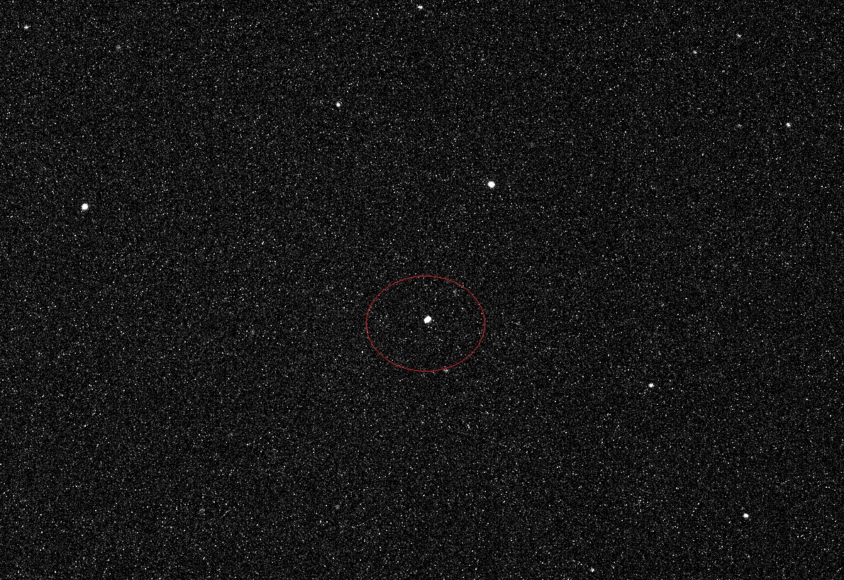
The satellite E-15 captured with 0.1 seconds of exposure, not showing any appreciable movement
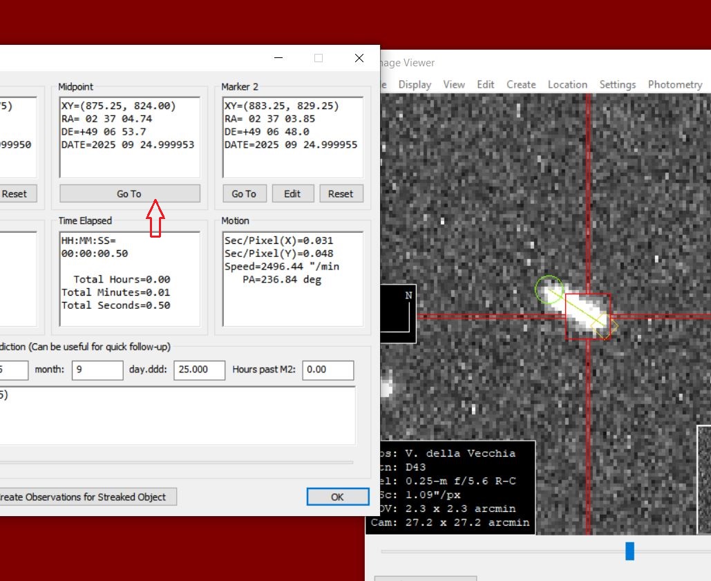
Creating a ruler and selecting midpoint in Tycho Tracker is very useful when longer exposure times are used (here, 0.5 sec)
It is now time to generate the astrometry for the satellite, which you do in the usual way. It’s better to create an ADES report rather than the MPC-80 columns as the former allows additional precision in timing, and to feed it to the proper page of the Project Pluto website. You will get an output like this:
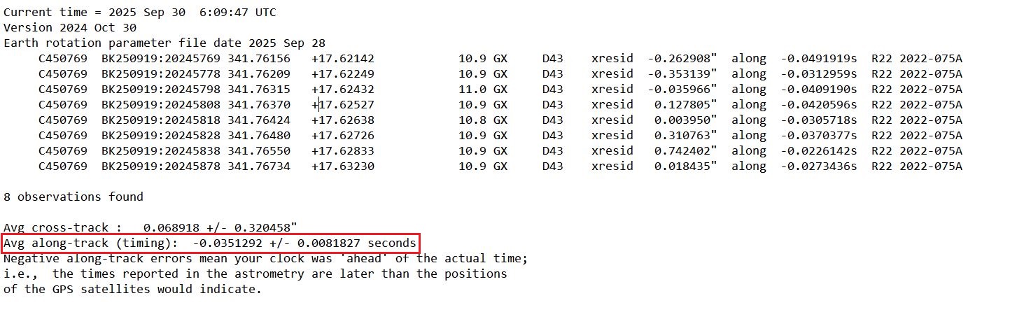
where the first columns are your observations, ending with observatory code. At the bottom, the average timing error is calculated (in red frame), in my case it is -0.03 seconds, while the other is the positional error. Better not rely on a single set of images, but to record at least 2 or 3 sessions targeting different satellites, averaging the timing offsets you get at the end. The timing error should be quite invariant if you keep constant all the imaging parameters as we have seen above.
Step 3: correct your observing time
At this point, you have to correct the date of your observations with the timing error you found. This can be done in imaging softwares like MaximDL (not free) or directly in the astrometric software like Tycho Tracker where this is quite straightforward.
In the Observatory settings menu, just select your Observatory and input the offset you found in Project Pluto with the same sign:
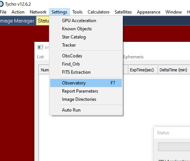
Tycho Tracker Observatory settings
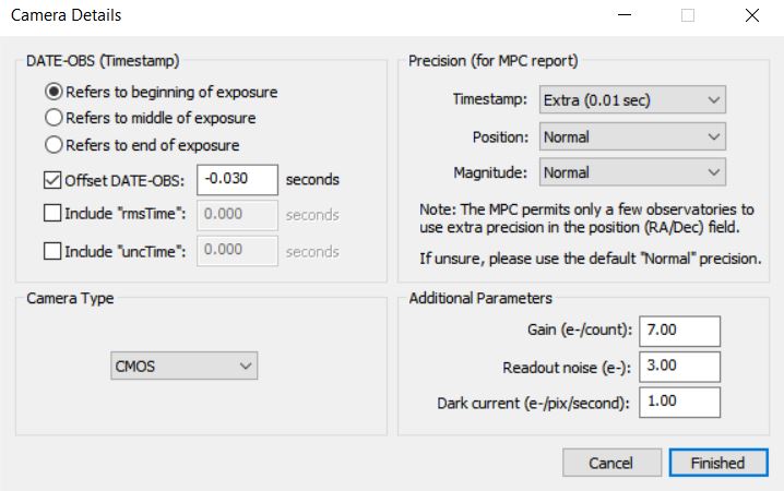
Input your timing offset as shown here
From now on, the software will add/subtract the indicated amount from the DATE-OBS field in your images before calculating the real observing time.
I recently had the chance to test my TimeBoxII+GNSS setup on the very fast NEO 2025 UC8, formerly on the NEOCP as ZTF1086. moving at 160″/minute at the time (late October 2025). At the time of writing, the orbit has an uncertainty of 1″, so residuals can change somehow in the future, nevertheless those from my Observatory are quite satisfying as you can see in the screenshot below, created with FindOrb.
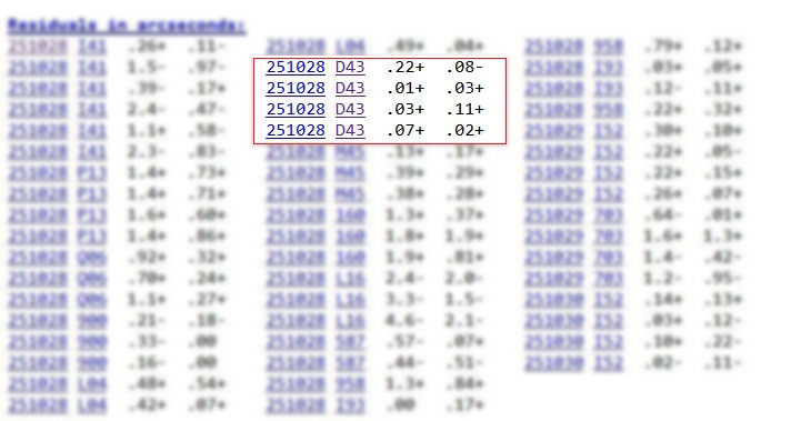
Residuals of the very fast NEO 2025 UC8 measured at my Observatory (D43)